TensorFlow中的CIFAR-10图像分类

在这篇文章中，我们将讨论如何使用TensorFlow对图像进行分类。图像分类是一种将图像分类到它们各自的类别的方法。CIFAR-10数据集，正如它所暗示的，其中有10个不同类别的图像。10个不同类别的图像共有60000张，分别是飞机、汽车、鸟、猫、鹿、狗、青蛙、马、船、卡车。所有图片的尺寸都是32×32。总共有50000张训练图像和10000张测试图像。

为了建立一个图像分类器，我们使用了 tensorflow 的keras API来建立我们的模型。为了建立一个模型，建议有GPU的支持，或者你也可以使用Google colab notebooks。

一步一步实现:

• 编写任何代码的第一步是导入所有需要的库和模块。这包括导入 tensorflow 和其他模块，如numpy。如果该模块不存在，那么你可以在命令提示符上使用pip install tensorflow下载它（对于windows），或者如果你使用的是jupyter笔记本，那么只需在单元格中输入！pip install tensorflow并运行它，以下载该模块。其他模块也可以用类似的方法导入。

import tensorflow as tf  

# Display the version
print(tf.__version__)    

# other imports
import numpy as np
import matplotlib.pyplot as plt
from tensorflow.keras.layers import Input, Conv2D, Dense, Flatten, Dropout
from tensorflow.keras.layers import GlobalMaxPooling2D, MaxPooling2D
from tensorflow.keras.layers import BatchNormalization
from tensorflow.keras.models import Model

输出:

2.4.1

上述代码的输出应该显示你所使用的tensorflow的版本，例如2.4.1或其他版本。

• 现在我们有了所需的模块支持，所以让我们加载我们的数据。CIFAR-10的数据集在tensorflow keras API上是可用的，我们可以使用 tensorflow.keras.datasets.cifar10 将其下载到我们的本地机器上，然后使用 load\_data() 函数将其分发到训练和测试集。

# Load in the data
cifar10 = tf.keras.datasets.cifar10

# Distribute it to train and test set
(x_train, y_train), (x_test, y_test) = cifar10.load_data()
print(x_train.shape, y_train.shape, x_test.shape, y_test.shape)

输出:

上述代码的输出将显示所有四个分区的形状，看起来会像这样

在这里，我们可以看到我们有5000张训练图像和1000张测试图像，如上所述，所有的图像都是32乘32的大小，有3个颜色通道，即图像是彩色图像。同时，我们也可以看到，每张图像都只有一个标签。

• 直到现在，我们的数据还在我们身边。但是，我们仍然不能将其直接发送到我们的神经网络。我们需要对数据进行处理，以便将其发送到网络中。这个过程中的第一件事是减少像素值。目前，所有的图像像素都在1-256的范围内，我们需要将这些值减少到0和1之间的数值。 这使我们的模型能够轻松地跟踪趋势和有效的训练。我们可以简单地通过将所有像素值除以255.0来做到这一点。

我们要做的另一件事是使用 flatten() 函数将标签值平移（简单地说就是以行的形式重新排列）。

# Reduce pixel values
x_train, x_test = x_train / 255.0, x_test / 255.0

# flatten the label values
y_train, y_test = y_train.flatten(), y_test.flatten()

• 现在是看到我们的数据集的一些图像的好时机。我们可以用子图的网格形式将其可视化。由于图片的大小只有32×32，所以不要对图片有太大的期望。它将是一个模糊的图像。我们可以使用matplotlib的subplot()函数来做可视化，并在训练数据集部分的前25张图片上循环。

# visualize data by plotting images
fig, ax = plt.subplots(5, 5)
k = 0

for i in range(5):
    for j in range(5):
        ax[i][j].imshow(x_train[k], aspect='auto')
        k += 1

plt.show()

输出:

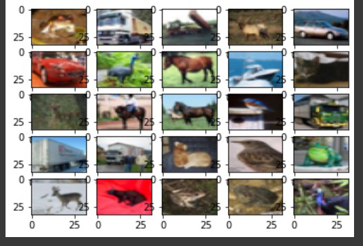
尽管这些图像并不清晰，但有足够的像素让我们明确这些图像中存在的物体。

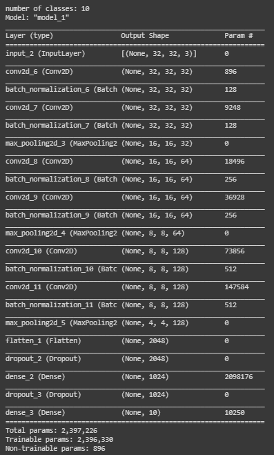
• 完成所有步骤后，现在是建立我们的模型的时候了。我们将使用卷积神经网络或CNN来训练我们的模型。它包括使用卷积层，也就是Conv2d层以及池化和归一化方法。最后，我们将把它传递到密集层和最后的密集层，也就是我们的输出层。我们使用的是’relu’激活函数。输出层使用 “softmax “函数。

# number of classes
K = len(set(y_train))

# calculate total number of classes
# for output layer
print("number of classes:", K)

# Build the model using the functional API
# input layer
i = Input(shape=x_train[0].shape)
x = Conv2D(32, (3, 3), activation='relu', padding='same')(i)
x = BatchNormalization()(x)
x = Conv2D(32, (3, 3), activation='relu', padding='same')(x)
x = BatchNormalization()(x)
x = MaxPooling2D((2, 2))(x)

x = Conv2D(64, (3, 3), activation='relu', padding='same')(x)
x = BatchNormalization()(x)
x = Conv2D(64, (3, 3), activation='relu', padding='same')(x)
x = BatchNormalization()(x)
x = MaxPooling2D((2, 2))(x)

x = Conv2D(128, (3, 3), activation='relu', padding='same')(x)
x = BatchNormalization()(x)
x = Conv2D(128, (3, 3), activation='relu', padding='same')(x)
x = BatchNormalization()(x)
x = MaxPooling2D((2, 2))(x)

x = Flatten()(x)
x = Dropout(0.2)(x)

# Hidden layer
x = Dense(1024, activation='relu')(x)
x = Dropout(0.2)(x)

# last hidden layer i.e.. output layer
x = Dense(K, activation='softmax')(x)

model = Model(i, x)

# model description
model.summary()

输出:

我们的模型现在已经准备好了，是时候对它进行编译了。我们正在使用model.compile()函数来编译我们的模型。对于参数，我们使用

• adam optimizer
• 稀疏分类交叉熵作为损失函数
• metrics=[‘accuracy’]

# Compile
model.compile(optimizer='adam',
              loss='sparse_categorical_crossentropy',
              metrics=['accuracy'])

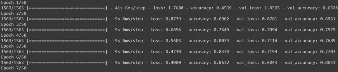
• 现在让我们用 model.fit() 来拟合我们的模型，把我们所有的数据传给它。我们将训练我们的模型到50个epochs，它给我们一个公平的结果，尽管你可以根据你的需要进行调整。

# Fit
r = model.fit(
  x_train, y_train, validation_data=(x_test, y_test), epochs=50)

输出:

该模型将开始训练，它将看起来像这样

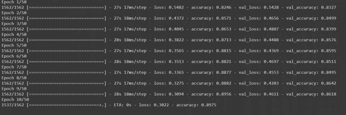
• 在这之后，我们的模型被训练了。虽然它可以正常工作，但为了使我们的模型更加准确，我们可以在我们的数据上添加数据增强，然后再次训练它。在增强的数据上再次调用model.fit()将继续训练它所离开的地方。我们将把我们的数据放在32个批次的大小上，我们将把宽度和高度的范围移动0.1，并水平地翻转图像。然后再次调用model.fit进行50个epochs。

# Fit with data augmentation
# Note: if you run this AFTER calling
# the previous model.fit()
# it will CONTINUE training where it left off
batch_size = 32
data_generator = tf.keras.preprocessing.image.ImageDataGenerator(
  width_shift_range=0.1, height_shift_range=0.1, horizontal_flip=True)

train_generator = data_generator.flow(x_train, y_train, batch_size)
steps_per_epoch = x_train.shape[0] // batch_size

r = model.fit(train_generator, validation_data=(x_test, y_test),
              steps_per_epoch=steps_per_epoch, epochs=50)

输出:

该模型将开始训练50个epochs。虽然它是在GPU上运行，但至少需要10到15分钟。

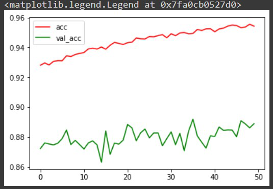
• 现在我们已经训练了我们的模型，在对它进行任何预测之前，让我们把每次迭代的准确率可视化，以便更好地分析。尽管还有其他的方法，包括混淆矩阵，以更好地分析模型。

# Plot accuracy per iteration
plt.plot(r.history['accuracy'], label='acc', color='red')
plt.plot(r.history['val_accuracy'], label='val_acc', color='green')
plt.legend()

输出:

让我们使用 model.predict() 函数对我们的模型中的图像进行预测。在将图像发送给我们的模型之前，我们需要再次减少0和1之间的像素值，并将其形状改为(1,32,32,3)，因为我们的模型希望输入只以这种形式存在。为了方便起见，让我们从数据集中抽取一张图片。它已经是缩小的像素格式，但我们仍然要用reshape()函数将其重塑为(1,32,32,3)。由于我们使用的是数据集的数据，我们可以比较预测的输出和原始输出。

# label mapping

labels = '''airplane automobile bird cat deerdog frog horseship truck'''.split()

# select the image from our test dataset
image_number = 0

# display the image
plt.imshow(x_test[image_number])

# load the image in an array
n = np.array(x_test[image_number])

# reshape it
p = n.reshape(1, 32, 32, 3)

# pass in the network for prediction and
# save the predicted label
predicted_label = labels[model.predict(p).argmax()]

# load the original label
original_label = labels[y_test[image_number]]

# display the result
print("Original label is {} and predicted label is {}".format(
    original_label, predicted_label))

输出:

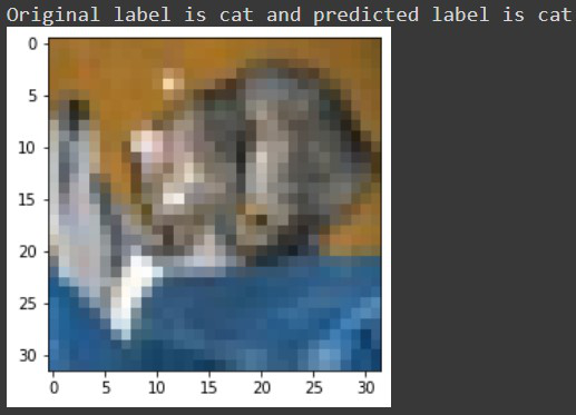
现在我们的输出是：原始标签是猫，预测的标签也是猫。

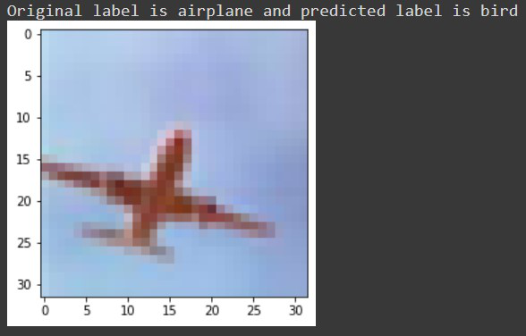
让我们对一些被我们的模型错误分类的标签进行检查，例如，对于5722号图像，我们收到这样的信息。

最后，让我们使用 model.save() 函数将我们的模型保存为h5文件。如果你使用的是Google collab，你可以从文件部分下载你的模型。

# save the model
model.save('geeksforgeeks.h5')

因此，通过这种方式，人们可以使用Tensorflow对图像进行分类。