用Python对服装图像进行分类

在社交媒体中，图片分类无处不在，从在Facebook、Instagram上挑选个人照片到在Myntra、Amazon、Flipkart等购物应用程序中对衣服图片进行分类。
分类已经成为任何电子商务平台的一个组成部分。分类也被用于识别法律和社交网络中的罪犯面孔。

在这篇文章中，我们将学习如何在Python中对图像进行分类。对服装图像进行分类是机器学习中图像分类的一个例子，它意味着将图像分类到它们各自的类别中。
为了获得服装图像，我们将使用TensorFlow中的fashion_mnist数据集。这个数据集包含10个不同类别的服装图像。它是初学者的MNIST数据集的替代品，由手写数字组成。我们将在接下来的工作中了解更多关于它的信息。

一步一步实现

第1步：为分类导入必要的库

• TensorFlow :使用python开发和训练模型
• NumPy:用于数组操作
• Matplotlib。用于数据可视化

# importing the necessary libraries
import tensorflow as tf
import numpy as np
import matplotlib.pyplot as plt

第2步：加载和探索数据

然后我们加载 fashion\_mnist 数据集，我们看到训练和测试数据的形状。很明显，有60,000张训练图片用于训练数据，10,000张测试图片用于测试模型。它总共包含10个类别的70,000张图片，即 “T恤/上衣”、”裤子”、”套头衫”、”连衣裙”、”外套”、”凉鞋”、”衬衫”、”运动鞋”、”包 “和 “踝靴”。

# storing the dataset path
clothing_fashion_mnist = tf.keras.datasets.fashion_mnist

# loading the dataset from tensorflow
(x_train, y_train),
(x_test, y_test) = clothing_fashion_mnist.load_data()

# displaying the shapes of training and testing dataset
print('Shape of training cloth images: ',
      x_train.shape)

print('Shape of training label: ',
      y_train.shape)

print('Shape of test cloth images: ',
      x_test.shape)

print('Shape of test labels: ',
      y_test.shape)

输出:

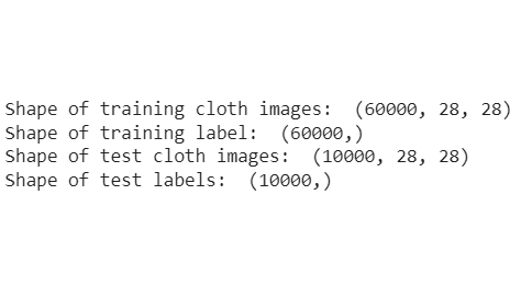
标签由一个从0到9的整数阵列组成。由于在 fashion\_mnist 数据集中没有添加类名，我们就把实际的类名存储在一个变量中，以便以后用于数据的可视化。
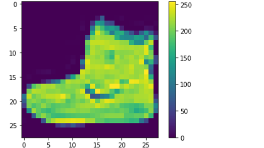
从输出结果来看，我们可以看到像素值在0到255的范围内。

# storing the class names as it is
# not provided in the dataset
label_class_names = ['T-shirt/top', 'Trouser',
                     'Pullover', 'Dress', 'Coat',
                     'Sandal', 'Shirt', 'Sneaker',
                     'Bag', 'Ankle boot']

# display the first images
plt.imshow(x_train[0]) 
plt.colorbar()  # to display the colourbar
plt.show()

输出:

第3步： 对数据进行预处理

下面的代码对数据进行了归一化处理，因为我们可以看到像素值落在0到255的范围内。
因此，我们需要用255除以0和1之间的值。

x_train = x_train / 255.0  # normalizing the training data
x_test = x_test / 255.0  # normalizing the testing data

第四步： 数据可视化

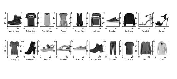
下面的代码显示了前20张服装图片和它们的类别标签，以确保我们在建立模型时方向正确。
在这里，我们将 x\_train与colormap 绘制成二进制，并从我们之前存储的 label\_class\_names 数组中添加了每个类别的名称。

plt.figure(figsize=(15, 5))  # figure size
i = 0
while i < 20:
    plt.subplot(2, 10, i+1)

    # showing each image with colourmap as binary
    plt.imshow(x_train[i], cmap=plt.cm.binary)

    # giving class labels
    plt.xlabel(label_class_names[y_train[i]])
    i = i+1

plt.show()  # plotting the final output figure

输出:

第五步： 建立模型

在这里，我们通过创建神经网络的层来建立我们的模型。
tf.keras.layer.Flatten() 将图像从二维数组转换为一维数组，tf.keras.layer.Dense ，有一定的参数，在训练阶段学习。

# Building the model
model = tf.keras.Sequential([
    tf.keras.layers.Flatten(input_shape=(28, 28)),
    tf.keras.layers.Dense(128, activation='relu'),
    tf.keras.layers.Dense(10)
])

第6步： 编译模型

这里我们使用adam优化器编译模型，SparseCategoricalCrossentropy 作为损失函数，并且 metrics=[‘准确性’] 。

# compiling the model
cloth_model.compile(optimizer='adam',
                    loss=tf.keras.losses.SparseCategoricalCrossentropy(
                        from_logits=True),
                    metrics=['accuracy'])

第7步： 对所建模型进行数据训练

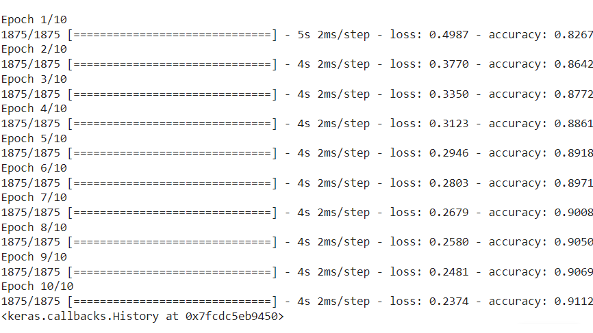
现在我们将把 x\_train 和 y\_train 即训练数据输入我们已经编译好的模型。model.fit() 方法有助于将训练数据装入我们的模型。

# Fitting the model to the training data
cloth_model.fit(x_train, y_train, epochs=10)

输出:

第8步： 评估模型的损失和准确性

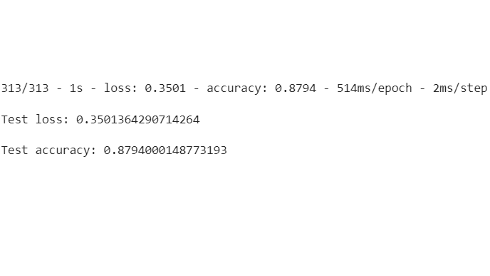
在这里，我们将通过计算模型的损失和准确性来了解我们的模型有多好。
从输出结果中，我们可以看到，测试数据的准确率低于训练数据的准确率。所以这是一个过拟合的模型。

# calculating loss and accuracy score
test_loss, test_acc = cloth_model.evaluate(x_test,
                                           y_test,
                                           verbose=2)
print('\nTest loss:', test_loss)
print('\nTest accuracy:', test_acc)

输出

第9步： 用测试数据对训练好的模型进行预测

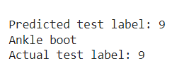
现在我们可以使用测试数据集来对建立的模型进行预测。我们尝试用 predictions[0] 来预测第一张测试图片，即 x\_test[0] ，结果是测试标签9，即Ankle boot。
我们添加了 Softmax() 函数，将线性输出对数转换为概率，因为它更容易计算。

# using Softmax() function to convert
# linear output logits to probability
prediction_model = tf.keras.Sequential(
    [cloth_model, tf.keras.layers.Softmax()])

# feeding the testing data to the probability
# prediction model
prediction = prediction_model.predict(x_test)

# predicted class label
print('Predicted test label:', np.argmax(prediction[0]))

# predicted class label name
print(label_class_names[np.argmax(prediction[0])])

# actual class label
print('Actual test label:', y_test[0])

输出:

第10步：预测与实际测试标签的数据可视化

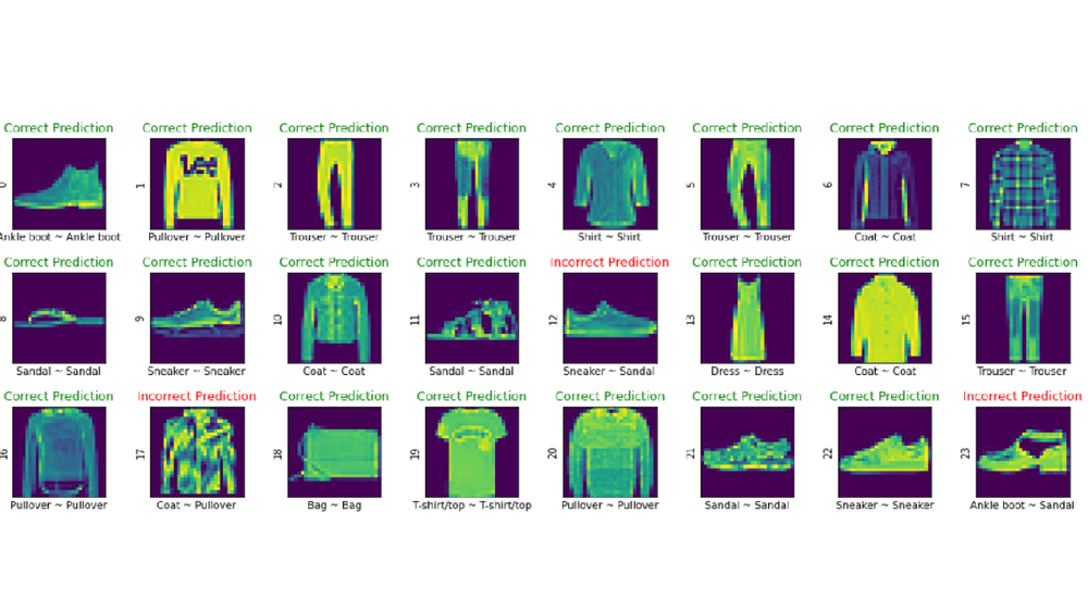
最后，我们将把我们的前24幅图像的预测与实际的类别标签进行可视化，看看我们的模型有多好。

# assigning the figure size
plt.figure(figsize=(15, 6))
i = 0

# plotting total 24 images by iterating through it
while i < 24:
    image, actual_label = x_test[i], y_test[i]
    predicted_label = np.argmax(prediction[i])
    plt.subplot(3, 8, i+1)
    plt.tight_layout()
    plt.xticks([])
    plt.yticks([])

    # display plot
    plt.imshow(image)

    # if else condition to distinguish right and
    # wrong
    color, label = ('green', 'Correct Prediction')
    if predicted_label == actual_label else (
        'red', 'Incorrect Prediction')

    # plotting labels and giving color to it
    # according to its correctness
    plt.title(label, color=color)

    # labelling the images in x-axis to see
    # the correct and incorrect results
    plt.xlabel(" {} ~ {} ".format(
        label_class_names[actual_label],
      label_class_names[predicted_label]))

    # labelling the images orderwise in y-axis
    plt.ylabel(i)

    # incrementing counter variable
    i += 1

输出:

我们可以清楚地看到，第12个、第17个和第23个预测的分类是错误的，但其余的是正确的。由于在现实中没有一个分类模型可以100%正确，这是我们建立的一个相当好的模型。